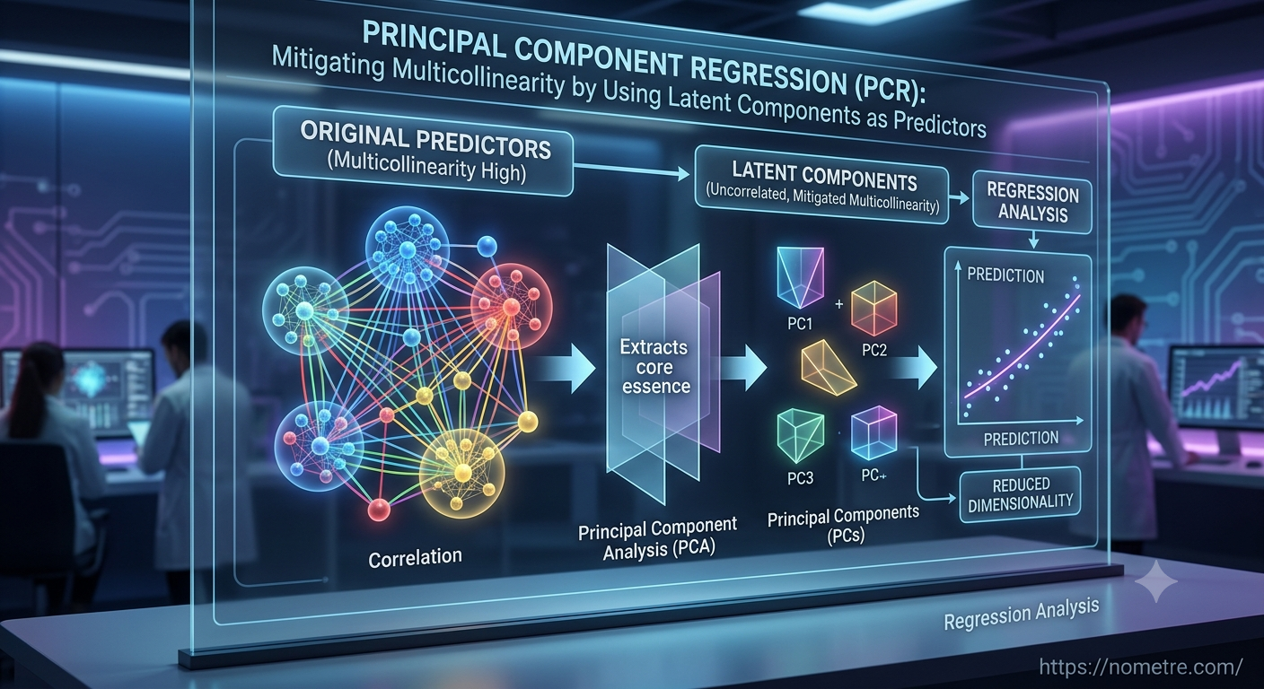
Multicollinearity is a common challenge in real-world regression problems. It happens when two or more predictor variables are highly correlated, making it difficult to estimate stable coefficients. In practice, you may see this in marketing data where spend across channels moves together, in finance where multiple indicators track the same economic trend, or in manufacturing where sensor readings overlap. When multicollinearity is present, a linear model can still predict reasonably well, but the coefficients become unreliable and sensitive to small changes in the dataset. This is where Principal Component Regression (PCR) becomes a practical technique.

PCR combines two ideas: dimensionality reduction through Principal Component Analysis (PCA) and regression on the reduced feature space. If you are learning regression modelling through a data scientist course, PCR is a helpful concept because it shows how you can improve model stability without abandoning linear methods. For learners coming from a data science course background, PCR also provides a clear bridge between unsupervised learning (PCA) and supervised learning (regression).

Why Multicollinearity Creates Problems in Regression

In ordinary least squares regression, the model estimates coefficients that minimise the squared prediction error. When predictors are strongly correlated, the model struggles to distinguish their individual effects. As a result:

• Coefficient estimates can swing widely with small changes in data.

• Standard errors inflate, making important predictors appear statistically insignificant.

• Interpretation becomes misleading, even if overall prediction error looks acceptable.

• Feature selection becomes unstable because correlated variables compete with each other.

In short, multicollinearity mainly harms interpretability and stability. PCR focuses on stability by replacing correlated variables with a smaller set of uncorrelated components.

The Core Idea Behind PCR

Principal Component Analysis transforms the original predictors into a new set of variables called principal components. Each component is a weighted combination of the original features. The key properties are:

• Components are orthogonal (uncorrelated with each other).

• The first few components capture most of the variation in the predictors.

• Later components capture less variation and are often closer to noise.

PCR then fits a regression model using the selected principal components instead of the original variables. Since the components are uncorrelated, multicollinearity is no longer an issue.

A practical way to think about PCR is: you are compressing your predictors into a smaller number of stable signals and then using those signals to predict the outcome.

Step-by-Step Workflow for Building a PCR Model

A good PCR workflow is systematic and easy to reproduce.

1) Standardise the predictors

PCA is sensitive to feature scale. Standardisation ensures that variables with larger ranges do not dominate the component construction. This step is almost always required unless all predictors share the same units and scale.

2) Apply PCA on the predictor matrix

Run PCA only on the X variables, not on the target. PCA identifies directions of maximum variance in the predictors. It does not consider which directions are most predictive of the outcome, which is an important limitation discussed later.

3) Choose the number of components

This is the most important decision in PCR. Common selection methods include:

• Explained variance threshold, such as keeping enough components to explain 90–95% of variance.

• Cross-validation, selecting the number of components that minimises prediction error on validation folds.

• A scree plot, looking for the “elbow” where additional components add limited value.

Cross-validation is usually the most reliable because it optimises the actual objective: predictive performance.

4) Fit regression using selected components

Once components are chosen, fit a linear regression model with these components as predictors. The model often becomes more stable and can generalise better, especially in high-dimensional or highly correlated datasets.

5) Evaluate and interpret carefully

PCR improves coefficient stability, but it changes interpretability. Coefficients now correspond to components, not original variables. If you need original-feature insights, you must map component loadings back to the feature space and interpret cautiously.

When PCR Works Well and When It Does Not

PCR is particularly useful in these settings:

• Many correlated predictors: For example, multiple survey questions measuring similar constructs.

• High-dimensional data: Where the number of predictors is large relative to sample size.

• Noise reduction: By dropping low-variance components, you may filter out some noise.

• Prediction-first problems: Where stable predictive performance matters more than direct interpretation.

However, PCR also has limitations:

• PCA ignores the target variable. A component that captures high variance in predictors may not be relevant for predicting the outcome. In some cases, a low-variance component could be highly predictive, and PCR may drop it.

• Interpretation becomes harder. Components are mixtures of features. Explaining business impact can be more complex than with standard regression.

• Not always best for feature selection. If interpretability is required, methods like ridge regression or elastic net may be preferred.

Because of these trade-offs, PCR is best seen as a robust tool in your modelling toolkit rather than the default choice.

Practical Learning Value for Data Professionals

PCR is commonly taught in advanced regression modules because it forces you to think about the relationship between variance, noise, and predictability. If you are building projects through a data scientist course in Pune, a strong PCR mini-project could involve comparing three models on the same dataset: ordinary least squares, ridge regression, and PCR, then explaining which one performs best under multicollinearity and why. For learners in a data science course, PCR helps you demonstrate applied understanding of both PCA and regression, which is a strong combination in interviews.

Conclusion

Principal Component Regression is a practical approach to mitigating multicollinearity by replacing correlated predictors with a smaller set of uncorrelated latent components. It improves model stability and can enhance generalisation, especially when predictors are many and strongly related. The key is to select components using cross-validation and to be realistic about interpretability. Used appropriately, PCR offers a clean, structured way to build reliable regression models in complex, real-world datasets.

BUSINESS DETAILS:

Name: Data Science, Data Analyst and Business Analyst Course in Pune
Address: First Floor, Sapphire Chambers, Spacelance Office Solutions Pvt. Ltd, 204, Baner Rd, Baner Gaon, Pune, Maharashtra 411069

Email Id: : enquiry@excelr.com
Phone Number: 9945850527